Introduction
What we are doing
- We have a dataset containing health indicators by county
- In the US, a "county" is an administrative unit that comprises multiple towns.
- In this case we want to see if there is a relationship between two of these health indicators; such as obesity and cardiac mortality rate.
- In order to expose that potential relationship we use a scatter plot, that display one valiable against the other.
Setup
Importing Modules
We start by importing the modules that will provide the basic functionalites for data manipulation and visualization.
Plotting Modules
Here we import the modules that support ploting functionalities.
The following command indicates that we want the plots to be shown "inline" (in the web page)
%matplotlib inline
Then we import "matplotlib". - This is a module that provides basic and advanced plotting functionalities. - More specifically, we import its "pylab" submodule. - We assign to it the alias "plt", to make easier for us to type subsequent commands.
from matplotlib import pylab as plt
Data Analysis Modules
We now import the "pandas" module. - It provides easy to use features for performing data analysis - It is well integrated with the plotting module - It provides support for reading data from many different file formats - We assign to it the alias "pd" to make easier for us to type commands later
import pandas as pd
We use the "read_csv" function from the pandas module, to read a csv ("comma separated") file containing the health indicators data.
df = pd.read_csv("indicators.csv")
Numerical Modules
Now we import the "numpy" module. - It provides support for numerical computation - In particular processing of vectors and matrices - We assign to it the alias "np" to make easier for us to type commands later
import numpy as np
Data Exploration
Data Frames
The pandas module reads data into a "Data Frame", which is essentially a matrix where the columns are identified by names and the rows are identified by indices.
Columns
Here we start by taking a look at the columns of the data frame to see how it is organized. This is a typical first step when we need to get familiar with the content of a new data file.
df.columns
Index([u'County Name', u'County Code', u'Region Name', u'Indicator Number', u'Indicator', u'Total Event Counts', u'Denominator', u'Denominator Note', u'Measure Unit', u'Percentage/Rate', u'95% CI', u'Data Comments', u'Data Years', u'Data Sources', u'Quartile', u'Mapping Distribution', u'Location'], dtype='object')
Index - Row names
We can also look at the names of the rows, also known as the "index". In this case, the index is a simple numerical ordering.
df.index
Int64Index([0, 1, 2, 3, 4, 5, 6, 7, 8, 9, 10, 11, 12, 13, 14, 15, 16, 17, 18, 19, 20, 21, 22, 23, 24, 25, 26, 27, 28, 29, 30, 31, 32, 33, 34, 35, 36, 37, 38, 39, 40, 41, 42, 43, 44, 45, 46, 47, 48, 49, 50, 51, 52, 53, 54, 55, 56, 57, 58, 59, 60, 61, 62, 63, 64, 65, 66, 67, 68, 69, 70, 71, 72, 73, 74, 75, 76, 77, 78, 79, 80, 81, 82, 83, 84, 85, 86, 87, 88, 89, 90, 91, 92, 93, 94, 95, 96, 97, 98, 99, ...], dtype='int64')
Pretty print
The pandas module provide a default pretty-print functionality that is also very helpful to get a sense of the content of the data frame. It has however the drawback that for data frames with many rows or many columns, scrolling may be needed to get a full picture of the data set. We invoke the pretty print by simply typing the name of the data frame.
df
County Name County Code Region Name Indicator Number \
0 Cayuga 5 Central New York d1
1 Cortland 11 Central New York d1
2 Herkimer 21 Central New York d1
3 Jefferson 22 Central New York d1
4 Lewis 23 Central New York d1
5 Madison 25 Central New York d1
6 Oneida 30 Central New York d1
7 Onondaga 31 Central New York d1
8 Oswego 35 Central New York d1
9 St. Lawrence 40 Central New York d1
10 Tompkins 50 Central New York d1
11 Central New York 103 Central New York d1
12 Chemung 7 Finger Lakes d1
13 Livingston 24 Finger Lakes d1
14 Monroe 26 Finger Lakes d1
15 Ontario 32 Finger Lakes d1
16 Schuyler 44 Finger Lakes d1
17 Seneca 45 Finger Lakes d1
18 Steuben 46 Finger Lakes d1
19 Wayne 54 Finger Lakes d1
20 Yates 57 Finger Lakes d1
21 Finger Lakes 102 Finger Lakes d1
22 Dutchess 13 Hudson Valley d1
23 Orange 33 Hudson Valley d1
24 Putnam 37 Hudson Valley d1
25 Rockland 39 Hudson Valley d1
26 Sullivan 48 Hudson Valley d1
27 Ulster 51 Hudson Valley d1
28 Westchester 55 Hudson Valley d1
29 Hudson Valley 106 Hudson Valley d1
30 Nassau 28 Nassau-Suffolk d1
31 Suffolk 47 Nassau-Suffolk d1
32 Nassau-Suffolk 108 Nassau-Suffolk d1
33 Bronx 58 New York City d1
34 Kings 59 New York City d1
35 New York 60 New York City d1
36 Queens 61 New York City d1
37 Richmond 62 New York City d1
38 New York City 107 New York City d1
39 Broome 3 New York-Penn d1
40 Chenango 8 New York-Penn d1
41 Tioga 49 New York-Penn d1
42 New York-Penn 104 New York-Penn d1
43 New York State 999 New York State d1
44 Albany 1 Northeastern New York d1
45 Clinton 9 Northeastern New York d1
46 Columbia 10 Northeastern New York d1
47 Delaware 12 Northeastern New York d1
48 Essex 15 Northeastern New York d1
49 Franklin 16 Northeastern New York d1
50 Fulton 17 Northeastern New York d1
51 Greene 19 Northeastern New York d1
52 Hamilton 20 Northeastern New York d1
53 Montgomery 27 Northeastern New York d1
54 Otsego 36 Northeastern New York d1
55 Rensselaer 38 Northeastern New York d1
56 Saratoga 41 Northeastern New York d1
57 Schenectady 42 Northeastern New York d1
58 Schoharie 43 Northeastern New York d1
59 Warren 52 Northeastern New York d1
... ... ... ...
Indicator Total Event Counts \
0 Cardiovascular disease mortality rate per 100,000 721
1 Cardiovascular disease mortality rate per 100,000 354
2 Cardiovascular disease mortality rate per 100,000 769
3 Cardiovascular disease mortality rate per 100,000 1023
4 Cardiovascular disease mortality rate per 100,000 238
5 Cardiovascular disease mortality rate per 100,000 522
6 Cardiovascular disease mortality rate per 100,000 2644
7 Cardiovascular disease mortality rate per 100,000 3607
8 Cardiovascular disease mortality rate per 100,000 1003
9 Cardiovascular disease mortality rate per 100,000 1019
10 Cardiovascular disease mortality rate per 100,000 593
11 Cardiovascular disease mortality rate per 100,000 12493
12 Cardiovascular disease mortality rate per 100,000 885
13 Cardiovascular disease mortality rate per 100,000 487
14 Cardiovascular disease mortality rate per 100,000 5766
15 Cardiovascular disease mortality rate per 100,000 935
16 Cardiovascular disease mortality rate per 100,000 204
17 Cardiovascular disease mortality rate per 100,000 274
18 Cardiovascular disease mortality rate per 100,000 943
19 Cardiovascular disease mortality rate per 100,000 721
20 Cardiovascular disease mortality rate per 100,000 223
21 Cardiovascular disease mortality rate per 100,000 10438
22 Cardiovascular disease mortality rate per 100,000 2293
23 Cardiovascular disease mortality rate per 100,000 2396
24 Cardiovascular disease mortality rate per 100,000 707
25 Cardiovascular disease mortality rate per 100,000 2305
26 Cardiovascular disease mortality rate per 100,000 709
27 Cardiovascular disease mortality rate per 100,000 1520
28 Cardiovascular disease mortality rate per 100,000 7449
29 Cardiovascular disease mortality rate per 100,000 17379
30 Cardiovascular disease mortality rate per 100,000 14166
31 Cardiovascular disease mortality rate per 100,000 11956
32 Cardiovascular disease mortality rate per 100,000 26122
33 Cardiovascular disease mortality rate per 100,000 10056
34 Cardiovascular disease mortality rate per 100,000 19966
35 Cardiovascular disease mortality rate per 100,000 10816
36 Cardiovascular disease mortality rate per 100,000 18237
37 Cardiovascular disease mortality rate per 100,000 4531
38 Cardiovascular disease mortality rate per 100,000 63606
39 Cardiovascular disease mortality rate per 100,000 2268
40 Cardiovascular disease mortality rate per 100,000 697
41 Cardiovascular disease mortality rate per 100,000 364
42 Cardiovascular disease mortality rate per 100,000 3329
43 Cardiovascular disease mortality rate per 100,000 164204
44 Cardiovascular disease mortality rate per 100,000 2669
45 Cardiovascular disease mortality rate per 100,000 562
46 Cardiovascular disease mortality rate per 100,000 715
47 Cardiovascular disease mortality rate per 100,000 646
48 Cardiovascular disease mortality rate per 100,000 347
49 Cardiovascular disease mortality rate per 100,000 478
50 Cardiovascular disease mortality rate per 100,000 620
51 Cardiovascular disease mortality rate per 100,000 510
52 Cardiovascular disease mortality rate per 100,000 58
53 Cardiovascular disease mortality rate per 100,000 694
54 Cardiovascular disease mortality rate per 100,000 618
55 Cardiovascular disease mortality rate per 100,000 1547
56 Cardiovascular disease mortality rate per 100,000 1664
57 Cardiovascular disease mortality rate per 100,000 1547
58 Cardiovascular disease mortality rate per 100,000 265
59 Cardiovascular disease mortality rate per 100,000 580
... ...
Denominator Denominator Note Measure Unit Percentage/Rate \
0 79763 Average annual population Rate 301.3
1 48898 Average annual population Rate 241.3
2 63638 Average annual population Rate 402.8
3 117619 Average annual population Rate 289.9
4 26772 Average annual population Rate 296.3
5 72254 Average annual population Rate 240.8
6 233403 Average annual population Rate 377.6
7 462913 Average annual population Rate 259.7
8 121905 Average annual population Rate 274.3
9 111116 Average annual population Rate 305.7
10 101689 Average annual population Rate 194.4
11 1439971 Average annual population Rate 289.2
12 88667 Average annual population Rate 332.7
13 64445 Average annual population Rate 251.9
14 741224 Average annual population Rate 259.3
15 107369 Average annual population Rate 290.3
16 18475 Average annual population Rate 368.1
17 34833 Average annual population Rate 262.2
18 98192 Average annual population Rate 320.1
19 92833 Average annual population Rate 258.9
20 25095 Average annual population Rate 296.2
21 1271131 Average annual population Rate 273.7
22 296350 Average annual population Rate 257.9
23 377072 Average annual population Rate 211.8
24 99636 Average annual population Rate 236.5
25 309006 Average annual population Rate 248.6
26 76758 Average annual population Rate 307.9
27 182127 Average annual population Rate 278.2
28 953658 Average annual population Rate 260.4
29 2294607 Average annual population Rate 252.5
30 1347132 Average annual population Rate 350.5
31 1503547 Average annual population Rate 265.1
32 2850679 Average annual population Rate 305.4
33 1391466 Average annual population Rate 240.9
34 2534814 Average annual population Rate 262.6
35 1605625 Average annual population Rate 224.5
36 2261761 Average annual population Rate 268.8
37 476976 Average annual population Rate 316.6
38 8270641 Average annual population Rate 256.4
39 198087 Average annual population Rate 381.7
40 50405 Average annual population Rate 460.9
41 50744 Average annual population Rate 239.1
42 299236 Average annual population Rate 370.8
43 19461584 Average annual population Rate 281.2
44 302018 Average annual population Rate 294.6
45 81897 Average annual population Rate 228.7
46 62421 Average annual population Rate 381.8
47 47018 Average annual population Rate 458.0
48 38746 Average annual population Rate 298.5
49 51141 Average annual population Rate 311.6
50 55255 Average annual population Rate 374.0
51 49041 Average annual population Rate 346.7
52 4851 Average annual population Rate 398.6
53 49584 Average annual population Rate 466.6
54 61926 Average annual population Rate 332.7
55 158122 Average annual population Rate 326.1
56 220186 Average annual population Rate 251.9
57 153985 Average annual population Rate 334.9
58 32285 Average annual population Rate 273.6
59 65853 Average annual population Rate 293.6
... ... ... ...
95% CI Data Comments Data Years \
0 NaN NaN 2009-2011
1 NaN NaN 2009-2011
2 NaN NaN 2009-2011
3 NaN NaN 2009-2011
4 NaN NaN 2009-2011
5 NaN NaN 2009-2011
6 NaN NaN 2009-2011
7 NaN NaN 2009-2011
8 NaN NaN 2009-2011
9 NaN NaN 2009-2011
10 NaN NaN 2009-2011
11 NaN NaN 2009-2011
12 NaN NaN 2009-2011
13 NaN NaN 2009-2011
14 NaN NaN 2009-2011
15 NaN NaN 2009-2011
16 NaN NaN 2009-2011
17 NaN NaN 2009-2011
18 NaN NaN 2009-2011
19 NaN NaN 2009-2011
20 NaN NaN 2009-2011
21 NaN NaN 2009-2011
22 NaN NaN 2009-2011
23 NaN NaN 2009-2011
24 NaN NaN 2009-2011
25 NaN NaN 2009-2011
26 NaN NaN 2009-2011
27 NaN NaN 2009-2011
28 NaN NaN 2009-2011
29 NaN NaN 2009-2011
30 NaN NaN 2009-2011
31 NaN NaN 2009-2011
32 NaN NaN 2009-2011
33 NaN NaN 2009-2011
34 NaN NaN 2009-2011
35 NaN NaN 2009-2011
36 NaN NaN 2009-2011
37 NaN NaN 2009-2011
38 NaN NaN 2009-2011
39 NaN NaN 2009-2011
40 NaN NaN 2009-2011
41 NaN NaN 2009-2011
42 NaN NaN 2009-2011
43 NaN NaN 2009-2011
44 NaN NaN 2009-2011
45 NaN NaN 2009-2011
46 NaN NaN 2009-2011
47 NaN NaN 2009-2011
48 NaN NaN 2009-2011
49 NaN NaN 2009-2011
50 NaN NaN 2009-2011
51 NaN NaN 2009-2011
52 NaN NaN 2009-2011
53 NaN NaN 2009-2011
54 NaN NaN 2009-2011
55 NaN NaN 2009-2011
56 NaN NaN 2009-2011
57 NaN NaN 2009-2011
58 NaN NaN 2009-2011
59 NaN NaN 2009-2011
... ... ...
Data Sources Quartile \
0 2009-2011 Vital Statistics Data as of February... 296.3 - < 350.5 : Q3
1 2009-2011 Vital Statistics Data as of February... 0 - < 296.3 : Q1 & Q2
2 2009-2011 Vital Statistics Data as of February... 350.5 + : Q4
3 2009-2011 Vital Statistics Data as of February... 0 - < 296.3 : Q1 & Q2
4 2009-2011 Vital Statistics Data as of February... 296.3 - < 350.5 : Q3
5 2009-2011 Vital Statistics Data as of February... 0 - < 296.3 : Q1 & Q2
6 2009-2011 Vital Statistics Data as of February... 350.5 + : Q4
7 2009-2011 Vital Statistics Data as of February... 0 - < 296.3 : Q1 & Q2
8 2009-2011 Vital Statistics Data as of February... 0 - < 296.3 : Q1 & Q2
9 2009-2011 Vital Statistics Data as of February... 296.3 - < 350.5 : Q3
10 2009-2011 Vital Statistics Data as of February... 0 - < 296.3 : Q1 & Q2
11 2009-2011 Vital Statistics Data as of February... NaN
12 2009-2011 Vital Statistics Data as of February... 296.3 - < 350.5 : Q3
13 2009-2011 Vital Statistics Data as of February... 0 - < 296.3 : Q1 & Q2
14 2009-2011 Vital Statistics Data as of February... 0 - < 296.3 : Q1 & Q2
15 2009-2011 Vital Statistics Data as of February... 0 - < 296.3 : Q1 & Q2
16 2009-2011 Vital Statistics Data as of February... 350.5 + : Q4
17 2009-2011 Vital Statistics Data as of February... 0 - < 296.3 : Q1 & Q2
18 2009-2011 Vital Statistics Data as of February... 296.3 - < 350.5 : Q3
19 2009-2011 Vital Statistics Data as of February... 0 - < 296.3 : Q1 & Q2
20 2009-2011 Vital Statistics Data as of February... 0 - < 296.3 : Q1 & Q2
21 2009-2011 Vital Statistics Data as of February... NaN
22 2009-2011 Vital Statistics Data as of February... 0 - < 296.3 : Q1 & Q2
23 2009-2011 Vital Statistics Data as of February... 0 - < 296.3 : Q1 & Q2
24 2009-2011 Vital Statistics Data as of February... 0 - < 296.3 : Q1 & Q2
25 2009-2011 Vital Statistics Data as of February... 0 - < 296.3 : Q1 & Q2
26 2009-2011 Vital Statistics Data as of February... 296.3 - < 350.5 : Q3
27 2009-2011 Vital Statistics Data as of February... 0 - < 296.3 : Q1 & Q2
28 2009-2011 Vital Statistics Data as of February... 0 - < 296.3 : Q1 & Q2
29 2009-2011 Vital Statistics Data as of February... NaN
30 2009-2011 Vital Statistics Data as of February... 296.3 - < 350.5 : Q3
31 2009-2011 Vital Statistics Data as of February... 0 - < 296.3 : Q1 & Q2
32 2009-2011 Vital Statistics Data as of February... NaN
33 2009-2011 Vital Statistics Data as of February... 0 - < 296.3 : Q1 & Q2
34 2009-2011 Vital Statistics Data as of February... 0 - < 296.3 : Q1 & Q2
35 2009-2011 Vital Statistics Data as of February... 0 - < 296.3 : Q1 & Q2
36 2009-2011 Vital Statistics Data as of February... 0 - < 296.3 : Q1 & Q2
37 2009-2011 Vital Statistics Data as of February... 296.3 - < 350.5 : Q3
38 2009-2011 Vital Statistics Data as of February... NaN
39 2009-2011 Vital Statistics Data as of February... 350.5 + : Q4
40 2009-2011 Vital Statistics Data as of February... 350.5 + : Q4
41 2009-2011 Vital Statistics Data as of February... 0 - < 296.3 : Q1 & Q2
42 2009-2011 Vital Statistics Data as of February... NaN
43 2009-2011 Vital Statistics Data as of February... NaN
44 2009-2011 Vital Statistics Data as of February... 0 - < 296.3 : Q1 & Q2
45 2009-2011 Vital Statistics Data as of February... 0 - < 296.3 : Q1 & Q2
46 2009-2011 Vital Statistics Data as of February... 350.5 + : Q4
47 2009-2011 Vital Statistics Data as of February... 350.5 + : Q4
48 2009-2011 Vital Statistics Data as of February... 296.3 - < 350.5 : Q3
49 2009-2011 Vital Statistics Data as of February... 296.3 - < 350.5 : Q3
50 2009-2011 Vital Statistics Data as of February... 350.5 + : Q4
51 2009-2011 Vital Statistics Data as of February... 296.3 - < 350.5 : Q3
52 2009-2011 Vital Statistics Data as of February... 350.5 + : Q4
53 2009-2011 Vital Statistics Data as of February... 350.5 + : Q4
54 2009-2011 Vital Statistics Data as of February... 296.3 - < 350.5 : Q3
55 2009-2011 Vital Statistics Data as of February... 296.3 - < 350.5 : Q3
56 2009-2011 Vital Statistics Data as of February... 0 - < 296.3 : Q1 & Q2
57 2009-2011 Vital Statistics Data as of February... 296.3 - < 350.5 : Q3
58 2009-2011 Vital Statistics Data as of February... 0 - < 296.3 : Q1 & Q2
59 2009-2011 Vital Statistics Data as of February... 0 - < 296.3 : Q1 & Q2
... ...
Mapping Distribution Location
0 2 (42.940095, -76.560755)
1 1 (42.597101, -76.143291)
2 3 (43.070026, -74.994246)
3 1 (44.019295, -75.898971)
4 2 (43.785537, -75.446296)
5 1 (42.986917, -75.720031)
6 3 (43.149482, -75.361773)
7 1 (43.065629, -76.168033)
8 1 (43.39123, -76.31133)
9 2 (44.689468, -75.242045)
10 1 (42.461024, -76.478784)
11 NaN NaN
12 2 (42.116644, -76.812331)
13 1 (42.763754, -77.765392)
14 1 (43.161748, -77.620143)
15 1 (42.894571, -77.252045)
16 3 (42.38593, -76.872032)
17 1 (42.833627, -76.82753)
18 2 (42.270053, -77.324618)
19 1 (43.144336, -77.117995)
20 1 (42.634338, -77.078311)
21 NaN NaN
22 1 (41.686216, -73.840468)
23 1 (41.422459, -74.241929)
24 1 (41.41131, -73.717443)
25 1 (41.127287, -74.017033)
26 2 (41.705166, -74.711705)
27 1 (41.848374, -74.099412)
28 1 (41.039278, -73.805386)
29 NaN NaN
30 2 (40.715749, -73.601185)
31 1 (40.820237, -73.119032)
32 NaN NaN
33 1 (40.85589, -73.868294)
34 1 (40.65642, -73.950691)
35 1 (40.726966, -74.005966)
36 1 (40.749338, -73.789673)
37 2 (40.566763, -74.148102)
38 NaN NaN
39 3 (42.122015, -75.933191)
40 3 (42.481798, -75.570013)
41 1 (42.120252, -76.29595)
42 NaN NaN
43 NaN NaN
44 1 (42.678066, -73.814233)
45 1 (44.731944, -73.548883)
46 3 (42.276913, -73.682168)
47 3 (42.242972, -74.997944)
48 2 (44.166026, -73.685145)
49 2 (44.705699, -74.340621)
50 3 (43.06014, -74.331296)
51 2 (42.298326, -73.973376)
52 3 (43.618468, -74.395268)
53 3 (42.933637, -74.341972)
54 2 (42.564852, -75.060334)
55 2 (42.70098, -73.628669)
56 1 (43.00894, -73.786779)
57 2 (42.809233, -73.946838)
58 1 (42.643426, -74.434606)
59 1 (43.403024, -73.716044)
... ...
[2733 rows x 17 columns]
Extracting Columns
It is common to find that not all columns of a data frame are relevant or interesting for our data analysis. Therefore it is desirable to extact the interesting columns out of the dataframe, in order to focus on them in the subsequent steps.
Column extraction is made by passing to the data frame a list of column names.
selectedColumns = ['County Name', 'County Code', 'Indicator Number', 'Indicator', 'Percentage/Rate']
df=df[selectedColumns]
Showing selected rows
The data frame head() function prints by default the first 5 records of the dataset. It is a useful way to take a look at how the data is organized.
df.head()
  County Name  County Code Indicator Number  \
0      Cayuga            5               d1
1    Cortland           11               d1
2    Herkimer           21               d1
3   Jefferson           22               d1
4       Lewis           23               d1

                                           Indicator  Percentage/Rate
0  Cardiovascular disease mortality rate per 100,000            301.3
1  Cardiovascular disease mortality rate per 100,000            241.3
2  Cardiovascular disease mortality rate per 100,000            402.8
3  Cardiovascular disease mortality rate per 100,000            289.9
4  Cardiovascular disease mortality rate per 100,000            296.3

[5 rows x 5 columns]
The head function also takes as argument the number of desired rows to print
df.head(3)
  County Name  County Code Indicator Number  \
0      Cayuga            5               d1
1    Cortland           11               d1
2    Herkimer           21               d1

                                           Indicator  Percentage/Rate
0  Cardiovascular disease mortality rate per 100,000            301.3
1  Cardiovascular disease mortality rate per 100,000            241.3
2  Cardiovascular disease mortality rate per 100,000            402.8

[3 rows x 5 columns]
Exploring Ranges
The pandas unique() function can be used to examine the unique values for a column. Let's illustrate this here, by first extracting a column (named 'Indicator') from the data frame, and then reducing the content of that column to the set of unique values.
The unique() function returns an array, so we us it to create a Series object, and then take advantage of its pretty-print functionality
indicators=pd.Series(df['Indicator'].unique())
indicators
0     Cardiovascular disease mortality rate per 100,000
1     Cerebrovascular disease (stroke) mortality rat...
2     Age-adjusted cerebrovascular disease (stroke) ...
3     Age-adjusted cardiovascular disease mortality ...
4                  Cirrhosis mortality rate per 100,000
5     Age-adjusted cirrhosis mortality rate per 100,000
6                   Diabetes mortality rate per 100,000
7      Age-adjusted diabetes mortality rate per 100,000
8     Age-adjusted percentage of adults with physici...
9     Age-adjusted percentage of adults with physici...
10    Percentage of pregnant women in WIC who were p...
11    Percentage of pregnant women in WIC who were p...
12    Percentage of WIC mothers breastfeeding at lea...
13    Percentage overweight but not obese (85th-<95t...
14    Percentage obese (95th percentile or higher) -...
15    Percentage overweight or obese (85th percentil...
16    Percentage overweight but not obese (85th-<95t...
17    Percentage obese (95th percentile or higher ) ...
18    Percentage overweight or obese (85th percentil...
19    Percentage overweight but not obese (85th-<95t...
20    Percentage obese (95th percentile or higher ) ...
21    Percentage overweight or obese (85th percentil...
22    Percentage obese (95th percentile or higher) c...
23    Percentage of children (aged 2-4 years) enroll...
24    Age-adjusted percentage of adults overweight o...
25    Age-adjusted percentage of adults obese (BMI 3...
26    Age-adjusted percentage of adults who did not ...
27    Age-adjusted percentage of adults eating 5 or ...
28    Cardiovascular disease hospitalization rate pe...
29            Cirrhosis hospitalization rate per 10,000
30    Age-adjusted cirrhosis hospitalization rate pe...
31    Diabetes hospitalization rate per 10,000 (prim...
32    Age-adjusted diabetes hospitalization rate per...
33    Diabetes hospitalization rate per 10,000 (any ...
34    Age-adjusted diabetes hospitalization rate per...
35    Age-adjusted cardiovascular disease hospitaliz...
36    Diabetes short-term complications hospitalizat...
37    Diabetes Short-term Complications Hospitalizat...
38    Cerebrovascular disease (stroke) hospitalizati...
39    Age-adjusted cerebrovascular disease (stroke) ...
dtype: object
Now that we have become familiar with the content of the data frame, we can proceed to generate plots of its values.
Plotting
We start our plotting exercise by selecting two specific health indicators. For them, we extract their rate of occurence for all the counties in the data set, and then we plot, per county, the rate of one indicator versus the other.
This is what would typically be done to explore potential correlations between two health indicators
Data Selection
From the list of unique health indicators, we choose two indicators of interest. We can do this by referring to them just by number.
indicator1=indicators[0]
indicator2=indicators[9]
We then print them out, as to verify which indicators we are plotting.
print "1: ",indicator1
print "2: ",indicator2
1:  Cardiovascular disease mortality rate per 100,000
2:  Age-adjusted percentage of adults with physician diagnosed diabetes
Data Extraction
Using each one of these indicators, we can now filter the data frame to extract the rows for which that specific indicator is present. We do this by taking advantage of a natural indexing provided by the pandas module.
data1=df[(df['Indicator']==indicator1)]
data2=df[(df['Indicator']==indicator2)]
We are essentially asking the data frame to return the list of records for which the value in the 'Indicator' column matches the specific value of one of our health indicators.
This produces two data frames, each one containing the data for that specific health indicator.
From them, we are particularly interested in the columns:
- County Name
- Percentage/Rate
We want to explore, for every county, how the percentage of occurrence of one health indicator, matches the percentage of occurence of the other health indicator. Again, we are exploring potential correlations between two health indicators.
Since the data is coming from a colection of records in a database, we must first extract them and index them by county, so that when we grab data from one indicator, we can be sure that we are matching it to another indicator for the same county.
data1_by_county = data1.set_index(data1['County Name'])
data2_by_county = data2.set_index(data2['County Name'])
Now that the indices are common, we can extract the column of data as a Series, for both indicators
rate1 = data1_by_county['Percentage/Rate']
rate2 = data2_by_county['Percentage/Rate']
Then we join both Series into a new Data Frame, and rename its columns to preserve the meaning of the health indicators
name1 = 'Cardiovascular'
name2 = 'Diabetes'

rates = pd.DataFrame([rate1,rate2],[name1,name2]).T
Real life data is messy. Here we can see that for some Counties we have missing data from one or both of the health indicators. We can drop those records from our analysis, using the dropna() function as follows
rates = rates.dropna()
And finally our data is organized in a consistent way, with two columns of data ready to be plot against each other in a scatter plot.
rates
                Cardiovascular  Diabetes
Albany                   294.6       8.6
Allegany                 313.9       8.7
Bronx                    240.9      11.3
Broome                   381.7       8.6
Cattaraugus              446.1      10.9
Cayuga                   301.3       9.5
Chautauqua               378.6      11.2
Chemung                  332.7      11.3
Chenango                 460.9      12.1
Clinton                  228.7      10.0
Columbia                 381.8       6.6
Cortland                 241.3      10.5
Delaware                 458.0       8.7
Dutchess                 257.9       9.7
Erie                     351.1      10.5
Essex                    298.5      10.4
Franklin                 311.6      11.7
Fulton                   374.0       8.0
Genesee                  340.6      13.2
Greene                   346.7       8.7
Hamilton                 398.6       8.0
Herkimer                 402.8      11.2
Jefferson                289.9      10.7
Kings                    262.6      10.5
Lewis                    296.3      10.4
Livingston               251.9       9.9
Madison                  240.8       7.4
Monroe                   259.3       8.9
Montgomery               466.6       7.7
Nassau                   350.5       5.9
New York                 224.5       6.1
New York State           281.2       9.0
Niagara                  415.4      10.2
Oneida                   377.6       8.8
Onondaga                 259.7       7.6
Ontario                  290.3       7.4
Orange                   211.8       6.9
Orleans                  352.0       8.1
Oswego                   274.3       9.9
Otsego                   332.7       6.6
Putnam                   236.5       6.4
Queens                   268.8      11.0
Rensselaer               326.1       9.3
Richmond                 316.6       8.5
Rockland                 248.6       8.0
Saratoga                 251.9       8.4
Schenectady              334.9       9.4
Schoharie                273.6       7.6
Schuyler                 368.1      10.3
Seneca                   262.2      10.7
St. Lawrence             305.7      10.8
Steuben                  320.1       7.9
Suffolk                  265.1       9.0
Sullivan                 307.9      10.4
Tioga                    239.1      10.7
Tompkins                 194.4       7.4
Ulster                   278.2       8.0
Warren                   293.6       9.8
Washington               280.2       8.1
Wayne                    258.9       8.6
                           ...       ...

[63 rows x 2 columns]
Let's Plot
From our prepared Data Frame, we now extract the respective columns as Series
rate1 = rates[name1]
rate2 = rates[name2]
and pass them as arguments to the Matplotlib scatter function, that will generate the scatter plot
plt.scatter(rate1,rate2)
<matplotlib.collections.PathCollection at 0x7f92ef730d90>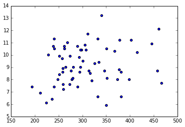
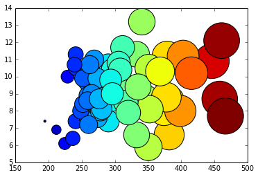
We can compare the values as well by using a bubble chart.
array1=np.array(rate1.tolist())
array1= array1[~np.isnan(array1)]
min=array1.min()
array_for_bubble=(array1-min+1)*10


plt.scatter(rate1, rate2, s=array_for_bubble, marker='o', c=array_for_bubble)
<matplotlib.collections.PathCollection at 0x7f92ef5cddd0>